KNN algorithm
The KNN algorithm is one of the data mining algorithms mainly used in data classification. This algorithm finds the k samples that are closest to the test sample from all the training data and calculates the average score of these k samples and considers them as the final estimated value for the test sample. The requirements of this algorithm include the following: first, we need to have samples with output or labeled data, second, we need a similarity unit or distance to calculate the distance between two samples, and third, we need to specify an Ak value. Determine the number of neighbors. KNN or WKNN algorithm is similar to KNA. For each test sample, each sample from the set of k obtained, how far from the test point, is set for that sample (coefficient). More distant ones have less effect on the result and closer samples have more effect16. First, the distance from the test sample to all training samples is calculated using Eq. (1)
$${D}_{i}={\left(\sum_{j=1}^{M}{\left|{X}_{ij}-{X}_{j}\right|}^{ 2}\right)}^{1/2}.$$
(1)
Equation (1) calculates the Euclidean distance of all samples from the test sample. which M; Number of features or inputs, Xij is the training sample, Xj is the test sample. Then the lowest values k obtained for the vector d are selected for the next step. The result of the test point can be expressed by Eq. (2)
$${C}_{un}=\frac{1}{k}\sum_{t=1}^{k}{C}_{t}.$$
(2)
Eq. (2), the value of C represents the label of the samples or the output value of the samples. This equation is used for KNN, but in WKNN, each coordinate axis is weighted relative to its distance from the experimental data. The value of this weight from Eq. (3)
$${w}_{i}=\frac{1/{D}_{i}}{{\sum }_{j=1}^{k}\left(1/{D}_{i} \right)}, i=\mathrm{1,2},\points,k.$$
(3)
Eq. (3), the variable w is the weight for each of the k samples. In the following, the final value is calculated based on the weights using Eq. (4)
$${C}_{un}=\sum_{i=1}^{k}{w}_{i}{C}_{i}.$$
(4)
Bee algorithm
The Bee algorithm was created in 2005. This algorithm simulates the feeding behavior in groups of bees17. Bees can be divided into three categories: foraging bees and foraging bees. A bee that goes to a predetermined food source is called a worker bee, a bee that randomly searches is called a forager, and a bee that moves around a dance area is called a forager. Choosing a leftover food source is called a foraging bee.
Firefly algorithm
Fireflies are a type of cockroach that emit a yellow and cool light through the process of bioluminescence. For a variety of reasons (such as differences in perception, such as breeding or defense mechanisms), night owls are more likely to go to a night owl that is brighter than themselves. The distance between night lights, the amount of ambient light absorption, the type of light source, and the amount of light emitted by the source are factors that affect the amount of light received from the source.
The firefly algorithm is an optimization method that mimics the behavior of a firefly and finds the optimal solution.18, 19, 20.
Multi-layered understanding
Neural networks are designed to create patterns that work like the human brain. A neural network works by creating an output pattern based on an input model provided to the network.21:22. Neural networks consist of a number of processing elements or neurons that receive and process input data and finally provide an output from it. Input data can be raw data or output from other neurons.23. The output can be the end product or input to other neurons. An artificial neural network consists of artificial neurons, which are actually functional elements. Each neuron has multiple inputs and assigned a weight to each input24, 25. The average output of each neuron is obtained from the sum of all inputs multiplied by the weights. The final result is achieved by applying the transformation function.
Multilayer perception or MLP is an architecture of artificial neural networks that divides the neurons of the network into multiple layers.26. In these networks, the first layer is the input, the last layer is the output, and the intermediate layers are called hidden layers.27. This architecture can be called the widely used architecture of neural networks.
Mixed methods
In this article, he developed a mixed method. This integrated method combines several methods such as FF, KNN, ABC, MLP and K-Means. In general, this integrated method is divided into three general parts and has two stages of training and testing. To increase the accuracy of the prediction, we use the data of 8 wells and use the K-Means clustering method to first put the wells with similar characteristics in one group, and then in the next block using the data of the wells at the time. t and in which group each hole belongs, the neural network estimates the result of the hole at time t + 1.
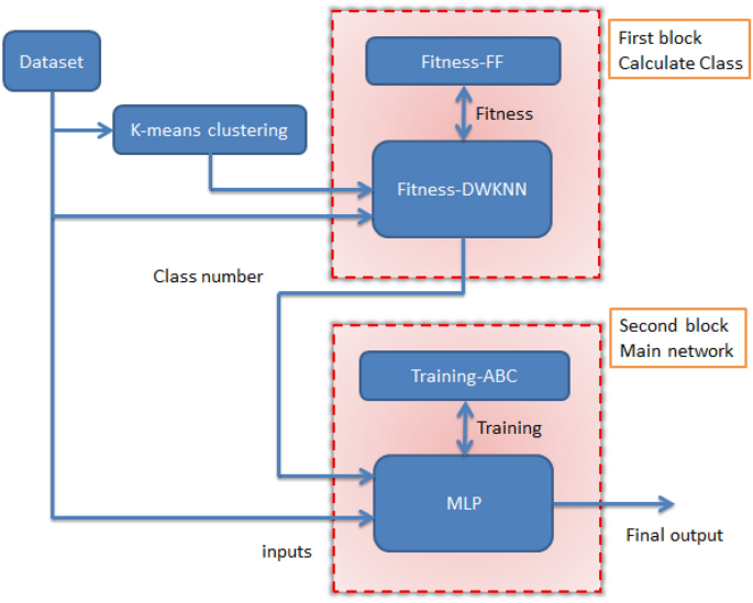
In the new method, the KNN method is used as the basic method for segmentation and the FF optimization algorithm is used to find the optimal control parameter of the input data. In addition, MLP was used to estimate the output values, and we used the ABC algorithm for better training. To perform the assignment we need to use a new result value that we define ourselves. So, we add a new output to the data set and find the value using the K-Means algorithm. The input data for the classification block is sent along with the new output. In the second step, when the components are determined, the data is sent to the second block to estimate the value. In this block, the ABC-MLP combination is used to estimate the value. For this block, the input values are sent with the new output. The control parameters used in this paper are listed in Table 1. Figure 1 shows the flow chart diagram of the training phase of the new method. The new method is developed in two stages: training and testing, and we will look at the training stage first.

General flow chart diagram of the training phase of the new method.
We need to use different information for each of the two levels. Therefore, we took 70% of the data as training data for the training phase and the remaining 30% as test data for the experimental phase. Based on 70% of the data we saw for the training class, we left 30% for verification.
Level of training
First, the data must be normalized, which is done using Eq. (5)
$${x}_{i}^{l}=\frac{{x}_{i}^{l}-min({x}^{l})}{max\left({x}^{ ) l}\right)-min({x}^{l})}\times 2-1.$$
(5)
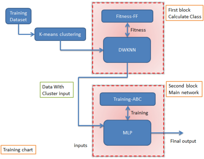
Eq. (5), the variable M is the quantity of inputs, xIl The ith sample is the lth input. Max(xl) value is the lth largest input number and min(xl) is the lth smallest input number. Figure 2 shows the block diagram associated with the training phase.

Flowchart diagram of the training phase of the new method.
After normalizing the data, we need to add a new parameter to the data, which specifies the number of the cluster or segment in which each data is located. We add that parameter to be used by the assignment block and increase the accuracy of the estimate. Determining which class each piece of data belongs to first blocks, but since the data is unlabeled and ungrouped, the number of classes and their data must be determined for this block first. Therefore, using the K-Means constraint, we first determine the maximum number of classes and data for each class. The Davies Bouldin value was used to find the optimal classes. This price is less, the number of units is the best (table 2).
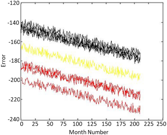
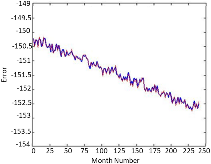
The smaller the Davis–Bouldin distance for ak , the more suitable the value of k . Therefore, for these 8 holes, the value is three clusters. Now, we divide all the data into three clusters using the K-Means algorithm and add a new output for each data, which stores the data segment number and has a value of one. It’s up to three. In Figure 3 you can see the closure of the wells. Figure 4 shows the confirmation of the well 1. This graph shows the great accuracy of the algorithm results. Additionally, show how this technique reduces noise in large data sets.

Data from 8 different wells were transformed into three clusters and displayed in three colors.

For good verification results 1.
To create three clusters from the eight-well data, we added a new column with the class number and values assigned between 1 and 3 based on the output of the K-Means algorithm. This operation was performed only during training, not during testing. The first block used data from scores 1, 2, and 3 for classification. To improve accuracy, we looked at combinations for each parameter using the Firefly method to determine the best value. Since optimization methods such as FireFly generate different solutions each time, due to optimal solutions, we obtained four weights with values of 0.1542987, 0.9254255, 0.4256712, and 0.6732144 from the best answers of the algorithm for the four inputs. All inputs have an equal impact on the output but may have different amounts based on their impact on the output value.
Error parameters
Equations (6) to (12) are given to determine the statistical comparison error of these algorithms. Based on the results presented in the results section and using these equations, we can compare the accuracy of the algorithm performance.
$${\mathrm{AE}}_{\mathrm{i}}=\frac{{\mathrm{S}}_{(\mathrm{measurable})}-{\mathrm{S}}_{(\ mathrm{estimated})}}{{\mathrm{S}}_{(\mathrm{measured})}}\times 100,$$
(6)
$$\mathrm{MAE}=\frac{{{\sum}_{\mathrm{i}=1}^{\mathrm{n}}\mathrm{PD}}_{\mathrm{i}}}{ \mathrm{n}},$$
(7)
$$\mathrm{MARE}=\frac{{\sum }_{\mathrm{i}=1}^{\mathrm{n}}\left|{\mathrm{PD}}_{\mathrm{i} }\right|}{\mathrm{n}},$$
(8)
$$\mathrm{STD}=\sqrt{\frac{{\sum }_{\mathrm{i}=1}^{\mathrm{n}}{({\mathrm{D}}_{\mathrm{ i}}-\mathrm{Dimean})}^{2}}{\mathrm{n}-1}},$$
(9)
$$\mathrm{Dimean}=\frac{1}{\mathrm{n}}\sum_{\mathrm{i}=1}^{\mathrm{n}}\left({{\mathrm{S}} ) _{\mathrm{measured}}}_{\mathrm{i}}-{{\mathrm{S}}_{\mathrm{predicted}}}_{\mathrm{i}}\right,$$
$$\mathrm{MSE}=\frac{1}{\mathrm{n}}\sum_{\mathrm{i}=1}^{\mathrm{n}}{\left({{\mathrm{S} ) }_{\mathrm{measured}}}_{\mathrm{i}}-{{\mathrm{S}}_{\mathrm{predicted}}_{\mathrm{i}}\right)}^{ 2},$$
(10)
$$\mathrm{RMSE}=\sqrt{\mathrm{MSE},}$$
(11)
$${\mathrm{R}}^{2}=1-\frac{\sum_{\mathrm{i}=1}^{\mathrm{N}}{({{\mathrm{S}}_{ \mathrm{predicted}}}_{\mathrm{i}}-{{\mathrm{S}}_{\mathrm{measured}}}_{\mathrm{i}}}}_{\mathrm{i} })}^{2}}{\sum_{\mathrm{i}=1}^{\mathrm{N}}{({{\mathrm{S}}_{\mathrm{Estimated}}}_{\ mathrm{i}}-\frac{{ \sum }_{\mathrm{I}=1}^{\mathrm{n}}{{\mathrm{S}}_{\mathrm{measurable}}}_{ \mathrm{i}}}{\mathrm {n}})}^{2}}.$$
(12)
[ad_2]
